


Why Order Quantity Divided by the Daily Target Is Not the Production Days: The Learning Curve and the Line Schedule
AI Process Analysis series · Supplement · Learning curve and production days
KEY POINTS
Work out production days as “order quantity ÷ daily target” and small orders come out too short while large orders come out too long. A new style starts at 40% of the target on day one and only reaches the target on day five. The gap changes with order quantity, factory, line splits and style changes, so no fixed correction can cover it, and the days have to be recalculated day by day whenever a condition changes.
Start with the most common calculation
When an order comes in, someone has to decide how many days to book on the line. The calculation most people use is this.
Production days = order quantity ÷ daily target
Example order DR-2026-001 is 3,000 pcs, and the daily target for this style at full speed is 496 pcs. So 3,000 ÷ 496 = 6.0 days, and the answer is a little over six days.
It is simple and intuitive, which is why it shows up in quotes, production plans and line schedule boards. But there is an assumption hidden in it: that the line makes exactly 496 pcs every day from the first day to the last.
On a sewing line, that assumption does not hold.
Two terms first
The daily target (Production Target) is the number of pieces a line makes in a day once it is fully used to the style and running at normal speed. In the example order it is 496 pcs. It comes from the SMV on the process analysis sheet, the number of operators and the factory efficiency, so it changes when the factory changes.
The learning curve is a curve showing that the same line with the same people produces a different amount on the first day of a new style than on the tenth.
Think of learning to drive. On the first day you take the same road slowly, and a few days later you cover it much faster. The road did not change, the driver got used to it. A sewing line works the same way. While dozens of operators get their hands around sewing motions they have never done and attachments they have never used, fewer pieces come out.
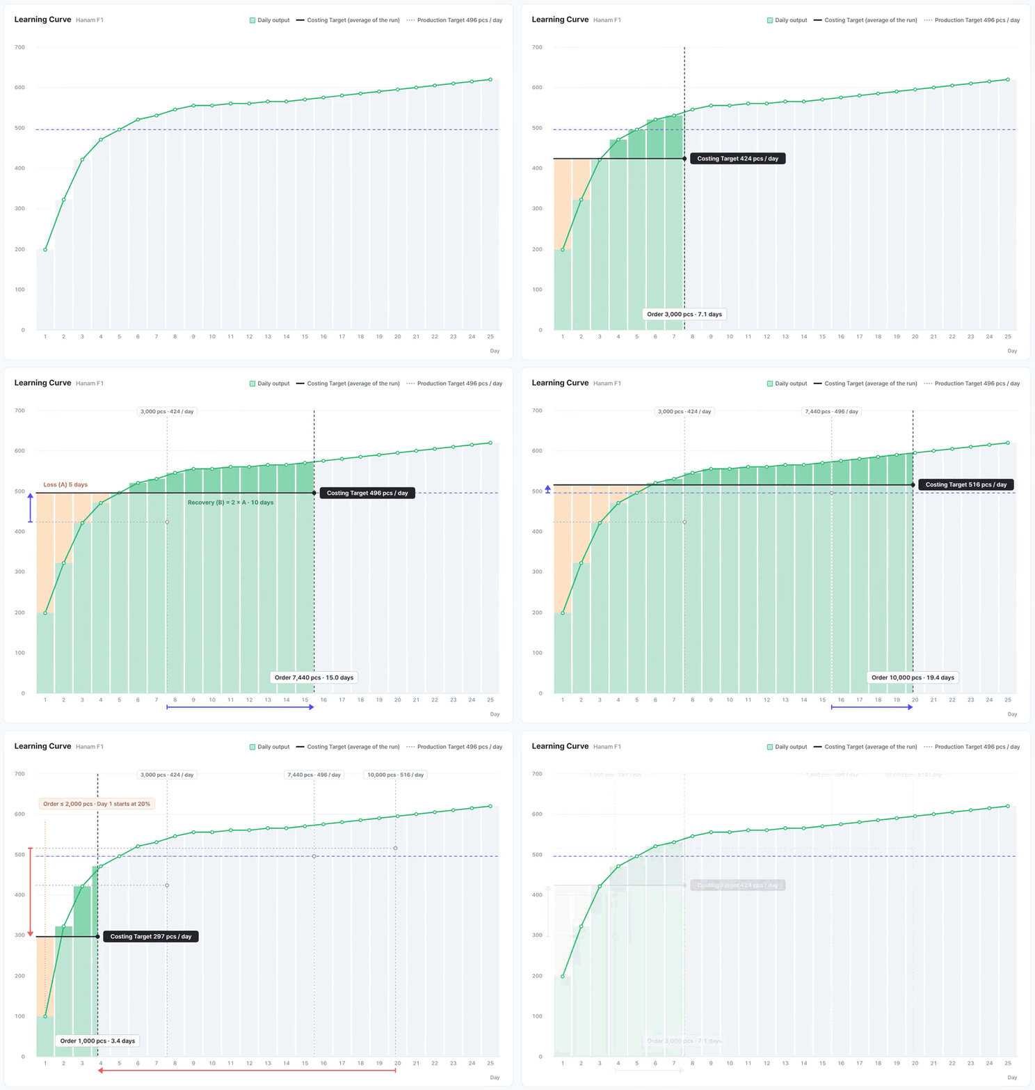
SIJE sets this curve as a percentage of the daily target. It is the standard rate covered in part 4. Day 1 is 40% of the daily target, day 2 is 65%, day 3 is 85%, day 4 is 95%, day 5 reaches 100%, and from day 6 the line makes a little more than the target.
Follow 3,000 pcs one day at a time
Let’s stack the same 3,000 pcs one day at a time in two ways. One is the plan that assumes 496 pcs every day, the other is the actual flow with the standard rate applied.
| Day | Rate | Output that day | Cumulative (actual flow) | Cumulative (496 pcs every day) |
|---|---|---|---|---|
| Day 1 | 40% | 198 pcs | 198 pcs | 496 pcs |
| Day 2 | 65% | 322 pcs | 521 pcs | 992 pcs |
| Day 3 | 85% | 422 pcs | 942 pcs | 1,488 pcs |
| Day 4 | 95% | 471 pcs | 1,414 pcs | 1,984 pcs |
| Day 5 | 100% | 496 pcs | 1,910 pcs | 2,480 pcs |
| Day 6 | 105% | 521 pcs | 2,430 pcs | 2,976 pcs |
| Day 7 | 107% | 531 pcs | 2,961 pcs | 3,472 pcs |
| Day 8 | 110% | 546 pcs | 3,507 pcs | 3,968 pcs |
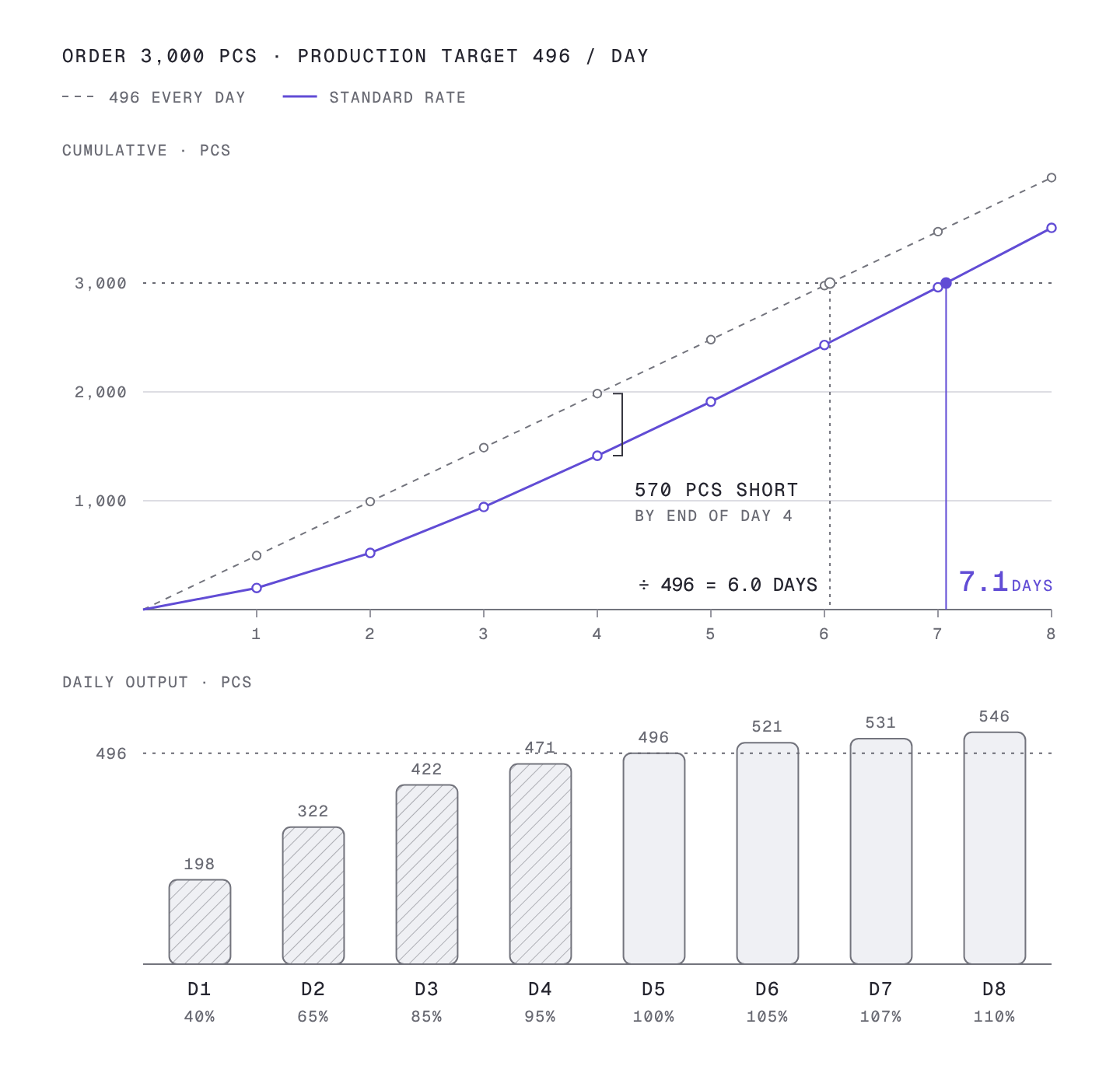
The plan that assumes 496 pcs a day gets close to 3,000 pcs around the end of day 6. The actual flow is at 2,430 pcs when day 6 ends, reaches 2,961 pcs only when day 7 ends, and fills 3,000 pcs early on day 8.
That is because the shortfall of the first four days piles up. On day 1 alone the line makes 298 pcs less than planned, and by day 4 the gap has grown to 570 pcs. Even when the line speeds up from day 5, a gap that size does not close quickly.
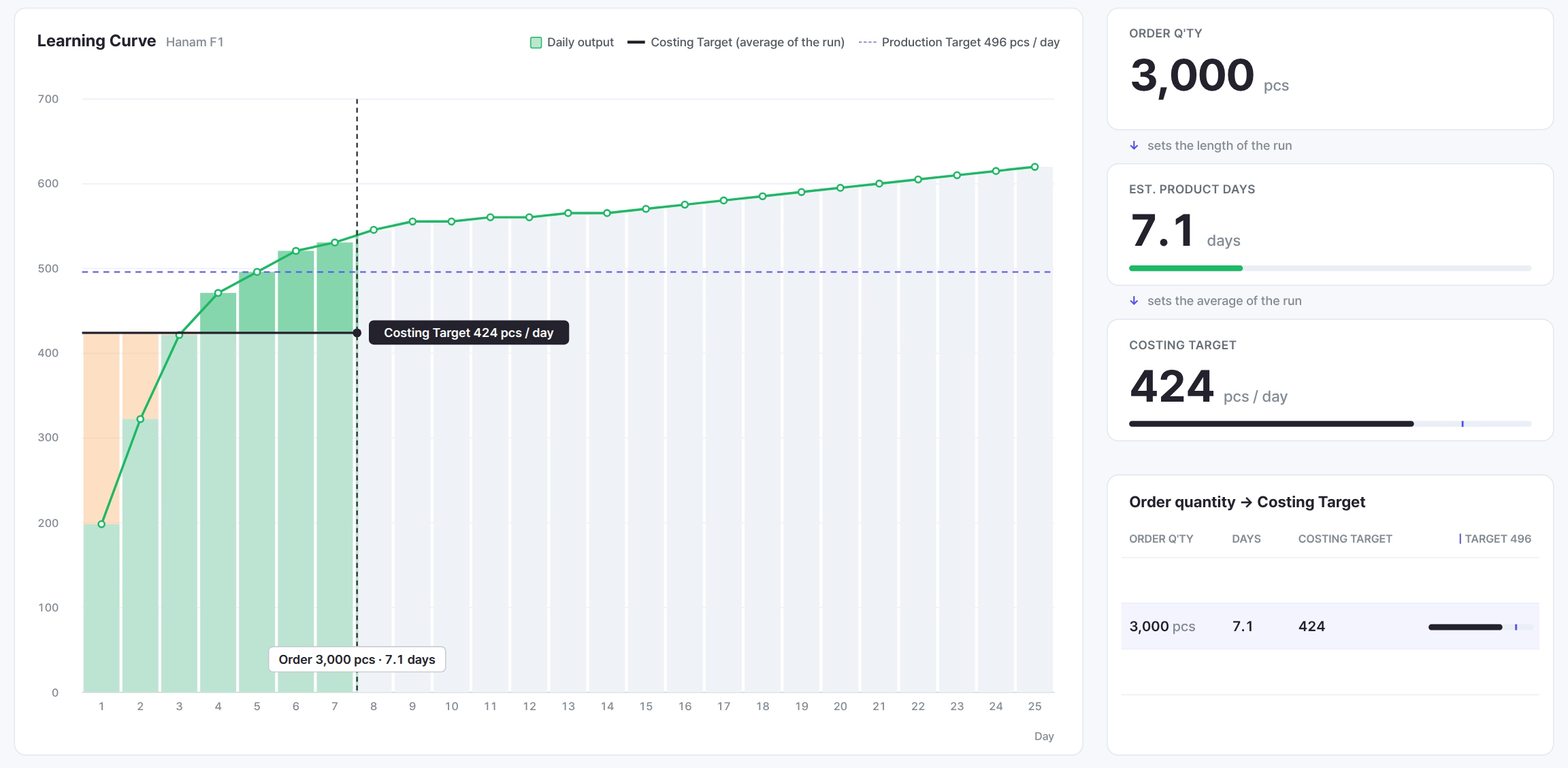
So the real production days for this order are 7.1, not 6.0. When the line schedule screen in part 5 booked this order on Hanam F1 line 3 from July 29 to August 5 as 7 working days, that number came from this calculation.
The average daily output over the whole order, slow days included, is called the Costing Target. In the example order it is 424 pcs, and 3,000 ÷ 424 = 7.1 days. In short, production days should be divided by this average, not by the daily target.
Then why not just “add a day”?
The usual fix is to add one day to the divided result. Look only at 3,000 pcs and it seems to work.
Change the quantity, though, and the fix stops working. These are the results for the same style, the same factory and the same daily target of 496 pcs, with only the quantity changed.
| Order quantity | Days by division (quantity ÷ 496) | Actual days with the learning curve | Actual average output (Costing Target) |
|---|---|---|---|
| 1,000 pcs | 2.0 days | 3.4 days | 297 pcs |
| 2,000 pcs | 4.0 days | 5.4 days | 372 pcs |
| 3,000 pcs | 6.0 days | 7.1 days | 424 pcs |
| 5,000 pcs | 10.1 days | 10.7 days | 468 pcs |
| 10,000 pcs | 20.2 days | 19.4 days | 516 pcs |
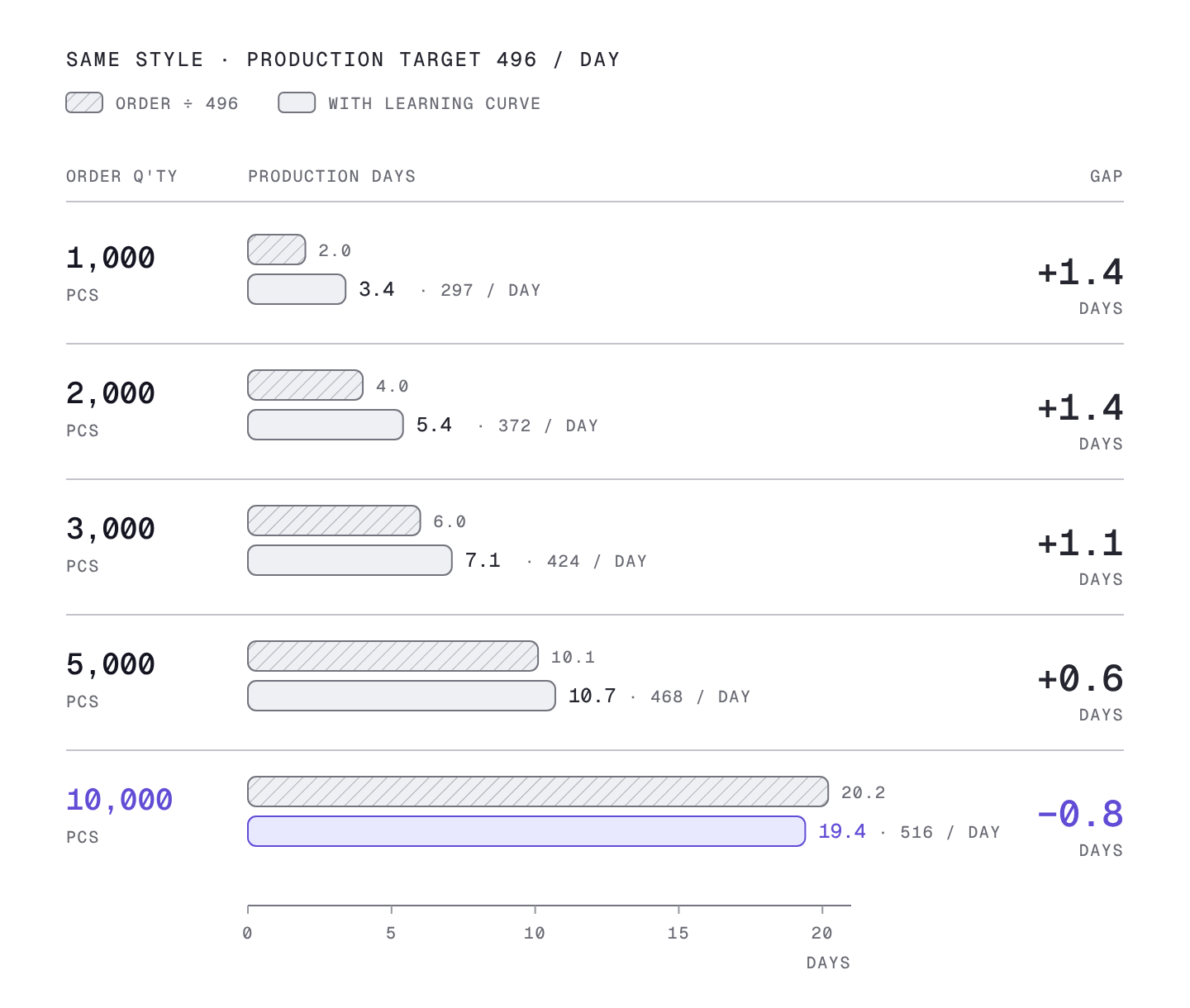
Read the table from top to bottom and three things show.
First, the smaller the order, the further the division falls short. 1,000 pcs is 2.0 days by division but actually takes 3.4 days. That is not one day short but close to a day and a half. The whole order ends inside the slow first few days.
Second, as the quantity grows the gap narrows. At 5,000 pcs the division gives 10.1 days and the actual figure is 10.7, a gap of a little over half a day. The days at normal speed get longer and dilute the loss of the first few days.
Third, at 10,000 pcs the direction flips. The division says 20.2 days, but the order actually finishes in 19.4. From day 6 the line makes more than the daily target for a long stretch, which pushes the average output of the whole order to 516 pcs, above the daily target of 496 pcs.
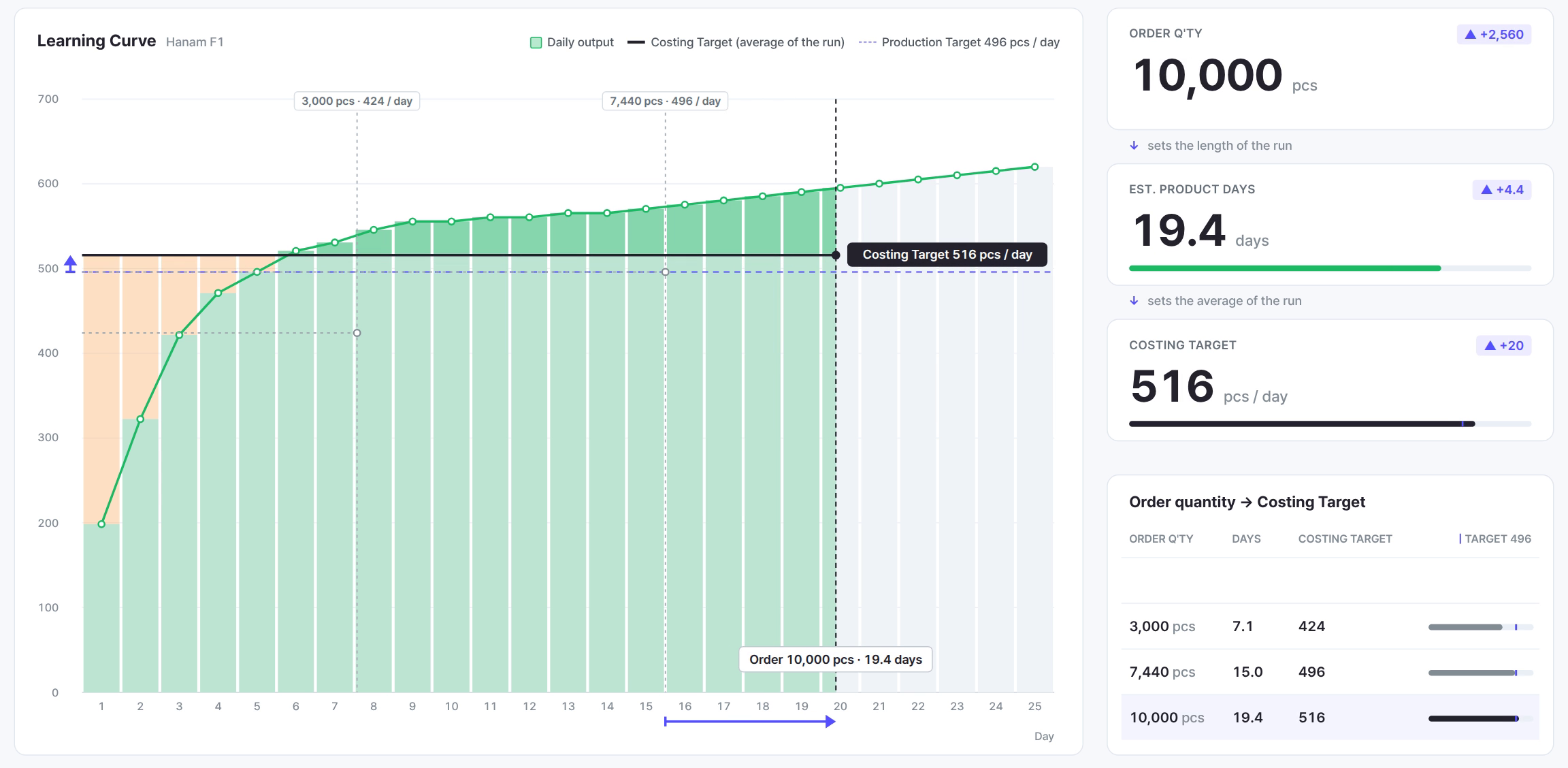
So the division is too short for small orders and too long for large ones. Add a day or add 10%, no single fixed correction fits every quantity.
Small orders start lower
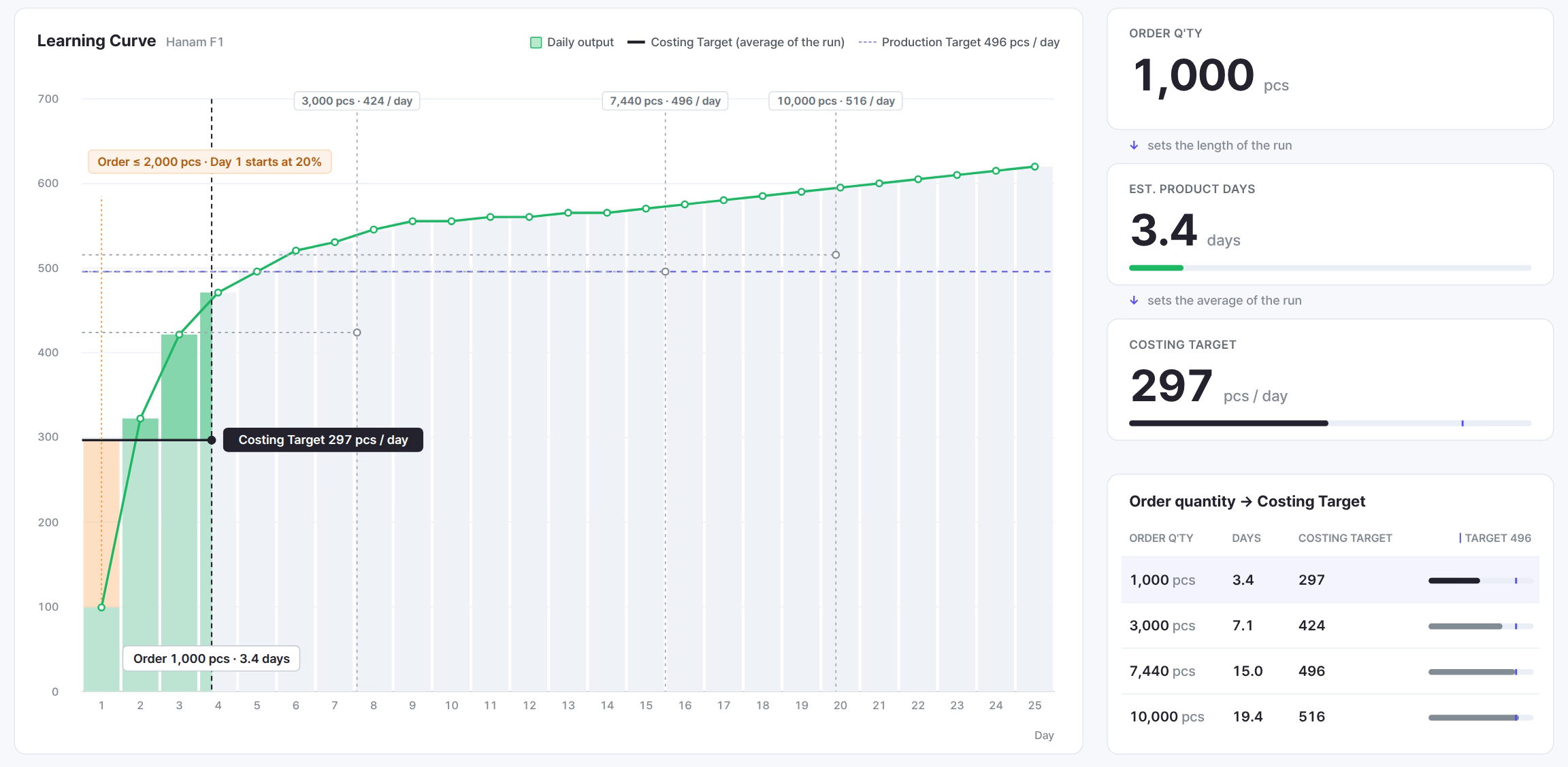
There is one more reason small orders are at a disadvantage. For orders of 2,000 pcs or less, day 1 starts at 20% instead of 40%.
The difference is not small. For the same 1,000 pcs, starting day 1 at 40% gives 3.1 days, and starting at 20% gives 3.4 days. Whether the quantity is above 2,000 pcs changes the starting point of the calculation itself.
Split the line or change the style and the curve starts over
So far the line has made one style from start to finish. A real line schedule is more complicated.
Take a line split first. If the delivery date is tight and 10,000 pcs is split into 5,000 pcs on each of two lines, the calendar shrinks from 19.4 days to 10.7. But both lines have to get used to the style again from day 1, so the average output per line drops from 516 pcs to 468 pcs. With each line tied up for 10.7 days, the factory as a whole uses more line days than it would running one line, and the CM goes up as the average output goes down.
Then a style change. Put three different 1,000 pcs styles on the same line one after another, and every change sends the line back to 20% on day 1, so you go through a 3.4-day order three times. The same 3,000 pcs made as one style takes 7.1 days, but split into three styles it ties up the line for much longer. This is why the schedule in a small-lot, high-mix factory always looks short.
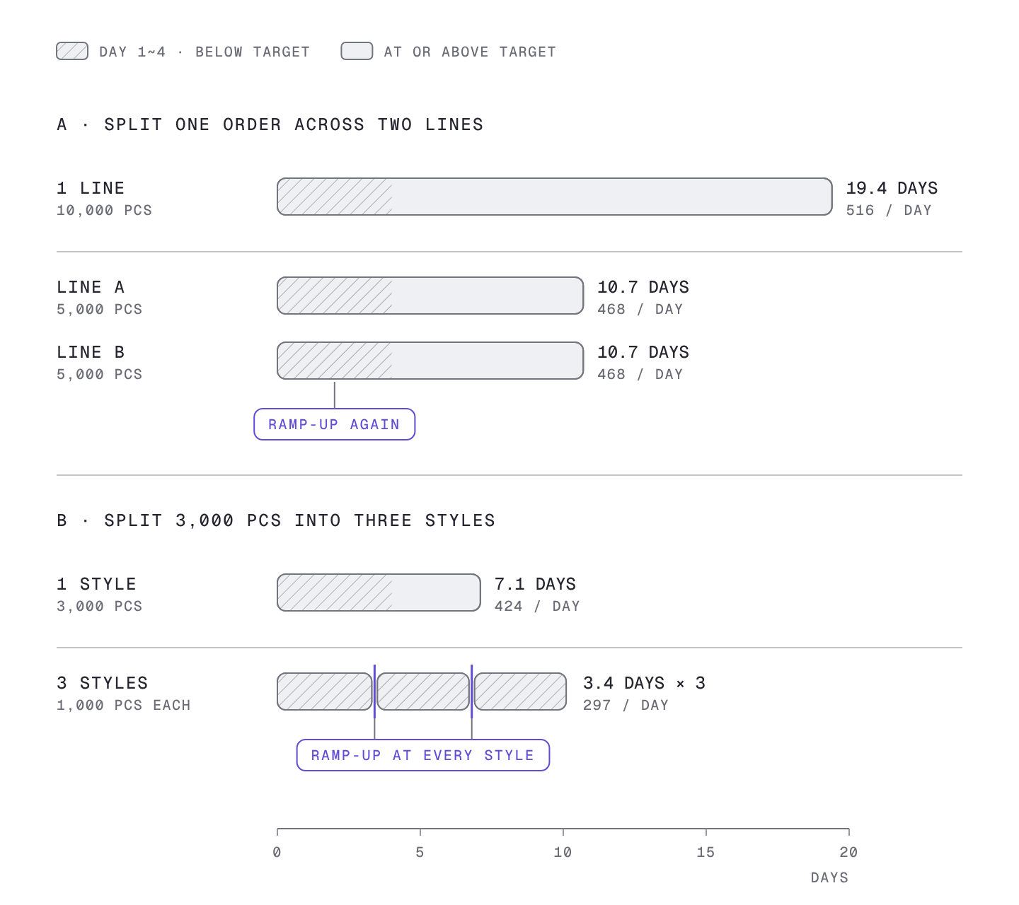
The other way round, if the same style comes in again right after, the second order starts with a line that already knows it and runs near 100% from the first day. The same quantity can take a different number of days depending on what order came before it.
If you want to calculate it in Excel
If you have followed this far, you can see what it takes to fill in one cell of production days.
- The daily target for each factory. Even with the same process analysis sheet, it changes with factory efficiency.
- A daily rate table. You need it day by day from day 1 until past normal speed.
- A starting point by order quantity. Day 1 changes depending on whether the order is 2,000 pcs or less.
- Cumulative output by day. Stack it one day at a time, find the day it reaches the order quantity, and work out what fraction of the last day is used.
- Line splits and style changes. At every point where the curve starts over, run the whole calculation again from the start.
Done once for one order, this can be handled in Excel. The trouble is that it has to be redone from scratch every time you try another factory at the quoting stage, every time the buyer changes the quantity, and every time you consider splitting a line for the delivery date. So on the floor this calculation gets skipped, the cells are filled in with quantity ÷ daily target, and the schedule that slips in the first week is patched up like an accident every time.
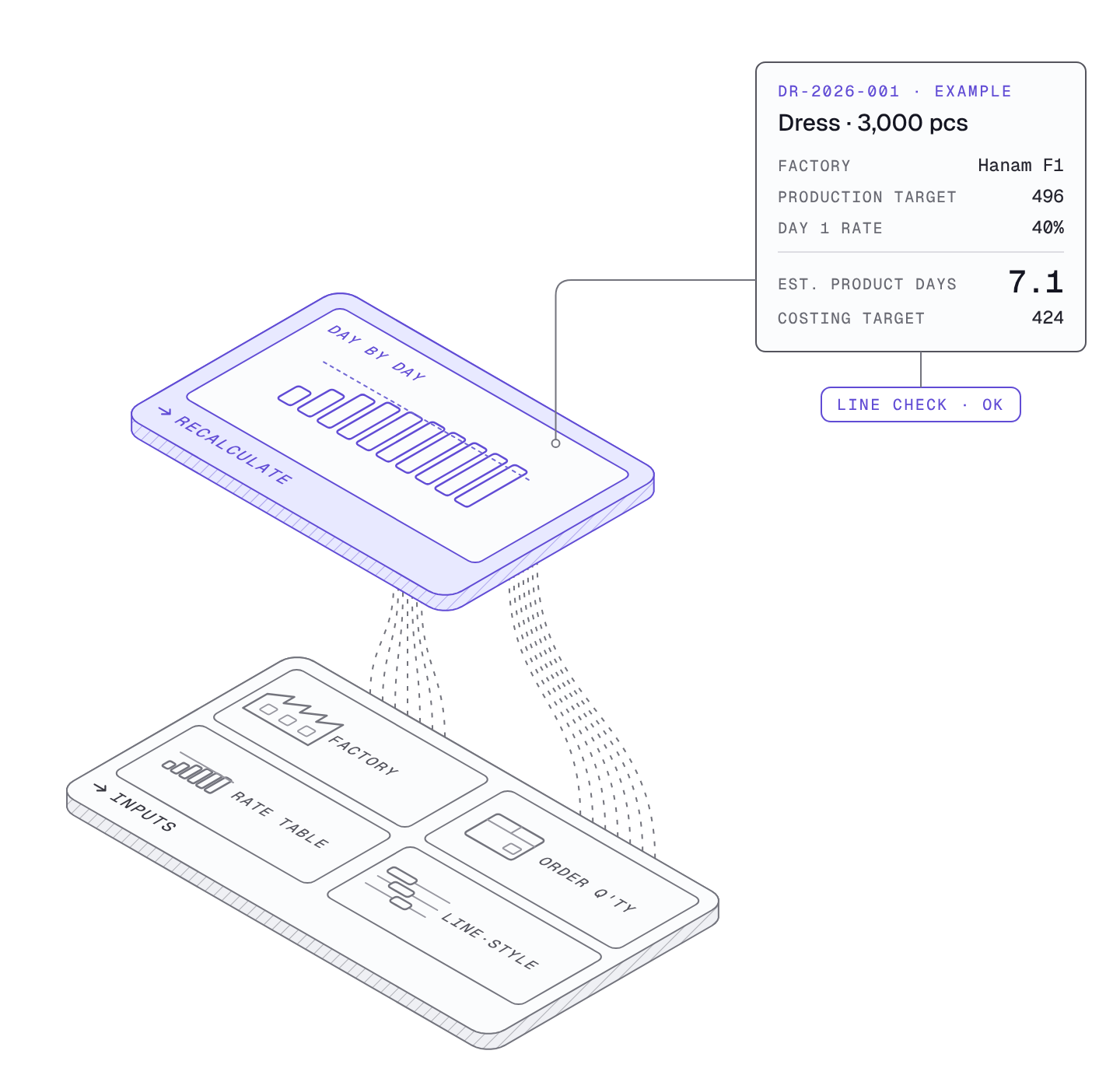
Monolis applies the standard rate day by day to the daily target that comes out of the process analysis sheet, and recalculates the actual production days and the Costing Target the moment the quantity or the factory changes. Those production days go straight into the line schedule check and come back as OK, Needs Adjustment or Not Feasible. The 7 working days on Hanam F1 line 3 in part 5 is a number produced this way.
Summary
| Question | By division | With the learning curve |
|---|---|---|
| How many days for 3,000 pcs | 6.0 days | 7.1 days |
| A small order (1,000 pcs) | 2.0 days | 3.4 days (1.4 days short) |
| A large order (10,000 pcs) | 20.2 days | 19.4 days (actually shorter) |
| Does adding a day fix it | Short or long depending on quantity | Recalculate for each quantity |
| Splitting the line | Days assumed to halve | The curve restarts on each line and the average output drops |
| Changing the style | Same quantity assumed to mean same days | Every style starts again from day 1 |
Production days are not a number you get from quantity and target alone. You get them only by calculating how the line gets used to the style. When the quoting figure and the schedule cells come from the same calculation, the schedule slips less in the first week.
Previous: Why the First Week Loses Money: Putting the Learning Curve into the Quote
Related: When the Lowest Unit Price Is Not the Optimal Factory: Checking the Line Schedule First
