


Where Does 40% on Day One Come From? Three Indicators That Define the Loss Zone of the Learning Curve
AI Process Analysis series · Supplement 2 · Three indicators of the loss zone
KEY POINTS
The front part of the learning curve, where the line falls short of its daily target, is the loss zone. It can be defined by three numbers: the start (the share of the daily target made on day 1), the reach day (the first day the line hits 100%), and the loss area (the total shortfall). What drives the quote and the schedule is the loss area, and the start and the reach day are the two conditions that set its size. SIJE’s standard curve is a starting value agreed so that vendors and factories can negotiate with the same numbers. It is adjusted by order quantity and repeat status, and it has to be recalibrated with measured data for each factory.
The question everyone asks about 40%
Parts 4 and Supplement 1 used SIJE’s standard rate throughout. On the first day a new style goes into a line, the line makes 40% of its daily target, then 65% on day 2, 85% on day 3 and 95% on day 4, and it reaches 100% on day 5.
Put this curve on the table in a quoting meeting and the question comes up: why exactly 40% on day one, and why does it reach 100% on day 5? A factory may push back that its lines climb faster. A vendor will want to know whether that number is solid enough to justify a higher CM (cut and make price).
Both sides are asking the same thing: where does this curve come from, and how far can it be trusted? This post answers in order. It starts with how the standard curve was set, then shows how to read the front of the curve as three indicators. After that come the inputs that change those indicators, and finally how a real factory’s curve differs from the standard and how to close that gap. All screens and figures are example data.
How the standard curve was set
Record the first two weeks of output for new styles across factories and styles for three years on the process analysis floor, and the curves do not converge on one line even inside the same factory. The same blouse runs differently in its first week with a collar and without one. The same style climbs at a different pace on a skilled line and on a line whose operators have just changed. A small order ends before the curve finishes climbing, and a line that made the same style a few weeks earlier starts high on day one. Style difficulty, line skill, order quantity and the gap since the previous order are all mixed into a single curve.
Pull one average line out of records that mix this many factors and you get a curve that fits no factory. So SIJE reversed the order. First it set a standard curve that vendors and factories can negotiate with in the same numbers, and then it layered factor adjustments and factory calibration on top. The standard rate of 40%, 65%, 85%, 95% and 100% is that standard curve.
This curve was not built as the right answer for every factory. It is a starting value that assumes it will be corrected with each factory’s measured data. Keep that in mind, and when we get to a real factory’s curve later, the gap reads as something to calibrate rather than an error.
Three numbers that define the loss zone
First, three terms. The daily target (Production Target) is the number of pieces a line makes in a day once it is fully used to the style and running at normal speed. In the example order in Supplement 1 it was 496 pcs. The rate is that day’s output written as a share of the daily target, and the loss zone is the days on which the rate is below 100%.
The shape of the loss zone can be set with three numbers.
The first is the start: what share of the daily target comes out on day 1. On the standard curve it is 40%, so with a daily target of 496 pcs the line is expected to make 198 pcs on day one.
The second is the reach day: the first day the line hits 100% of its daily target. On the standard curve it is day 5. This is the day that fixes what part 4 called the loss period A, because the line falls short from day 1 to day 4 and makes its full target for the first time on day 5.
The third is the loss area: the shortfall against the daily target, added up day by day. The calculation is simple. Subtract each day’s rate from 100% and add up the differences.
Loss area = (100% − day 1 rate) + (100% − day 2 rate) + … + (100% − rate on the last day below target)
On the standard curve the line is short by 60% on day 1, 35% on day 2, 15% on day 3 and 5% on day 4, so 60 + 35 + 15 + 5 = 115%. Over the first four days it makes 1.15 days’ worth of target less than planned.
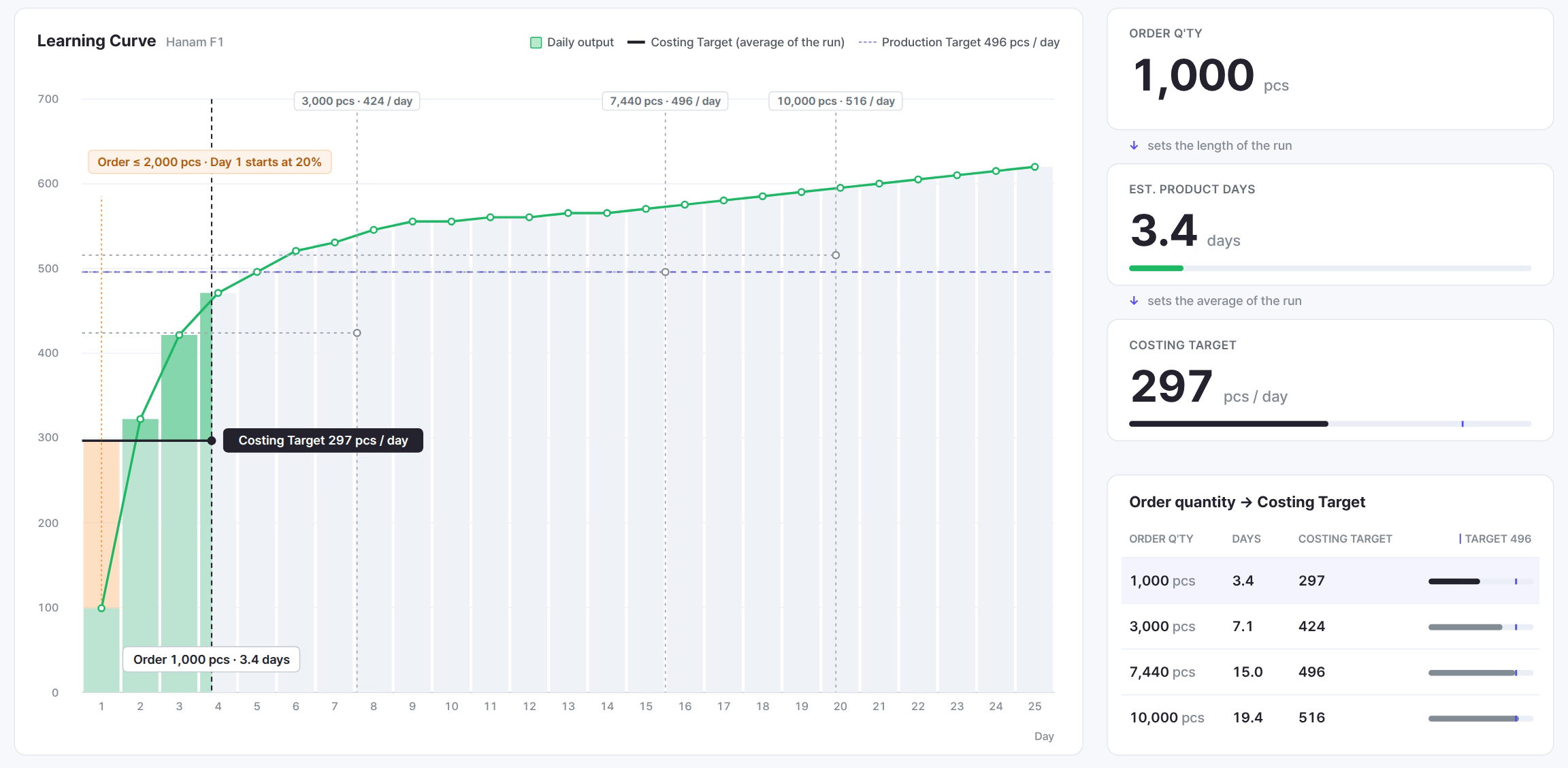
Turn the percentage into pieces and it becomes easier to picture. In Supplement 1, stacking a 3,000 pcs order day by day at a daily target of 496 pcs, the line made 298 pcs less than planned on day 1 alone, and by day 4 the gap had grown to 570 pcs. Those 570 pcs are the 115% loss area written in pieces.
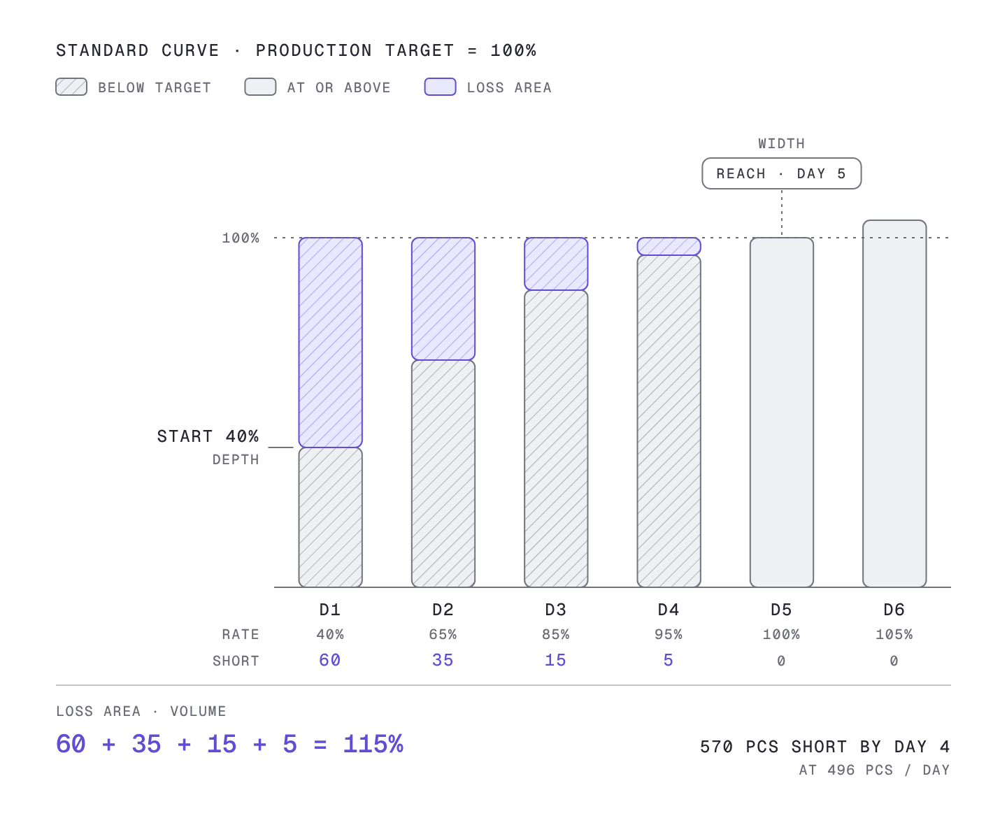
A puddle makes the relationship between the three numbers easy to see. The start is the depth of the puddle, the reach day is its width, and the loss area is the amount of water in it. With the same depth, a wider puddle holds more water, and with the same width, a deeper one holds more. The loss area is the result of both the start and the reach day, so changing either one changes the area.
The loss area is what changes the quote and the schedule
Of the three numbers, the loss area has the biggest effect on the quote, because the pieces not made do not disappear. They have to be paid back later.
This is where the 1:2 rule from part 4 comes in. Once the line gets used to the style, days come when it makes more than its daily target. On the standard curve the line goes a little over target day after day, 105% on day 6 and 107% on day 7. The stretch where this extra output pays back the earlier shortfall is the recovery zone, and the 1:2 rule holds that the recovery zone has to be twice as long as the loss zone to cover the loss.
On the standard curve it works out like this. Add up the output above target from day 6 to day 15: 5 + 7 + 10 + 12 + 12 + 13 + 13 + 14 + 14 + 15 = 115%. That matches the 115% lost earlier exactly. So on day 15 cumulative output catches up with cumulative target, and that day is the break-even day. Five days of loss, ten days of recovery, fifteen days in total. The 115% loss area sets break-even on day 15.
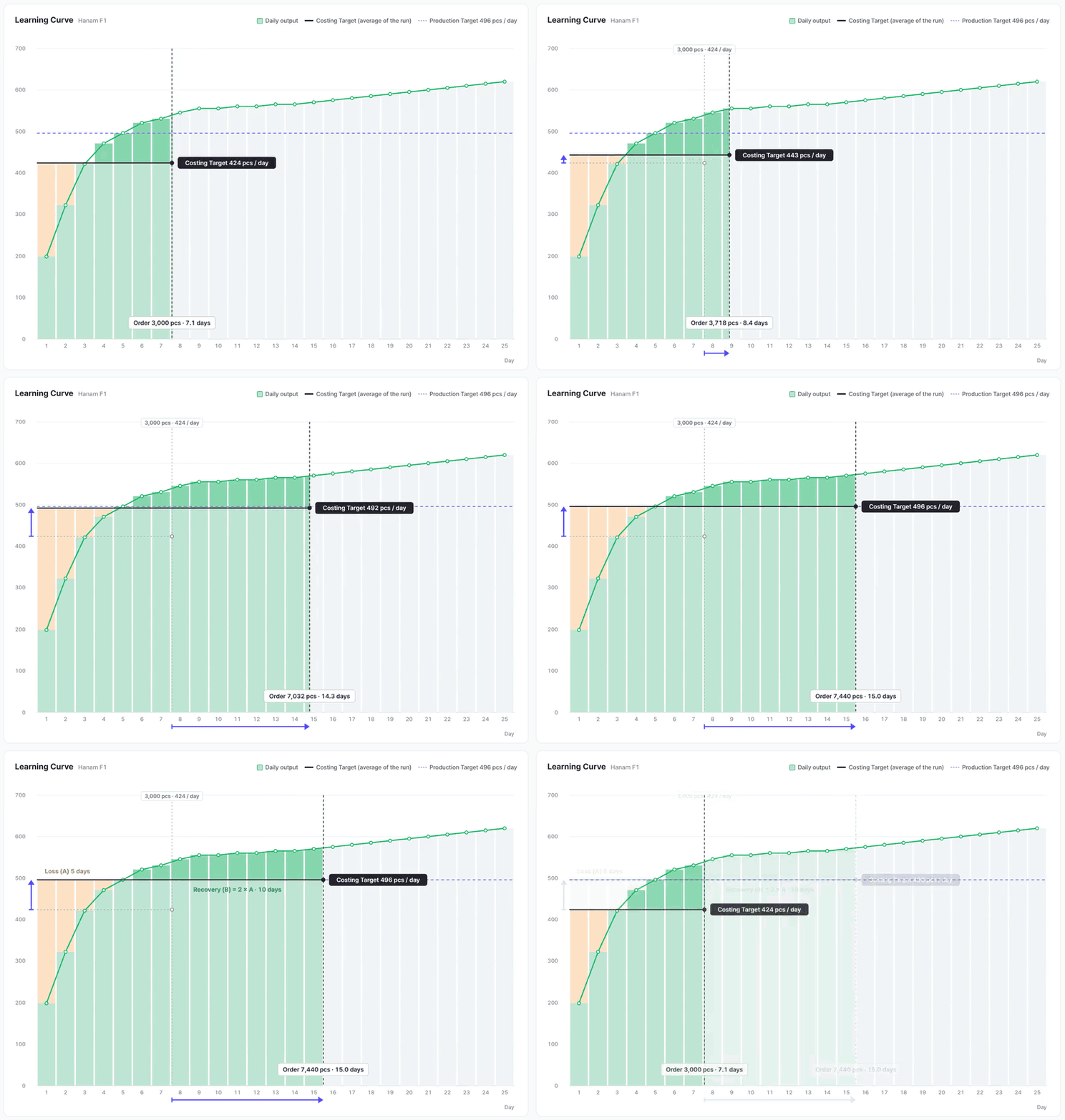
You can see this point directly on the Monolis learning curve screen. Set the order quantity to 7,440 pcs and production days come to 15.0, and the Costing Target becomes 496 pcs, the same as the daily target. It is the order size at which five days of loss and ten days of recovery cancel out exactly.
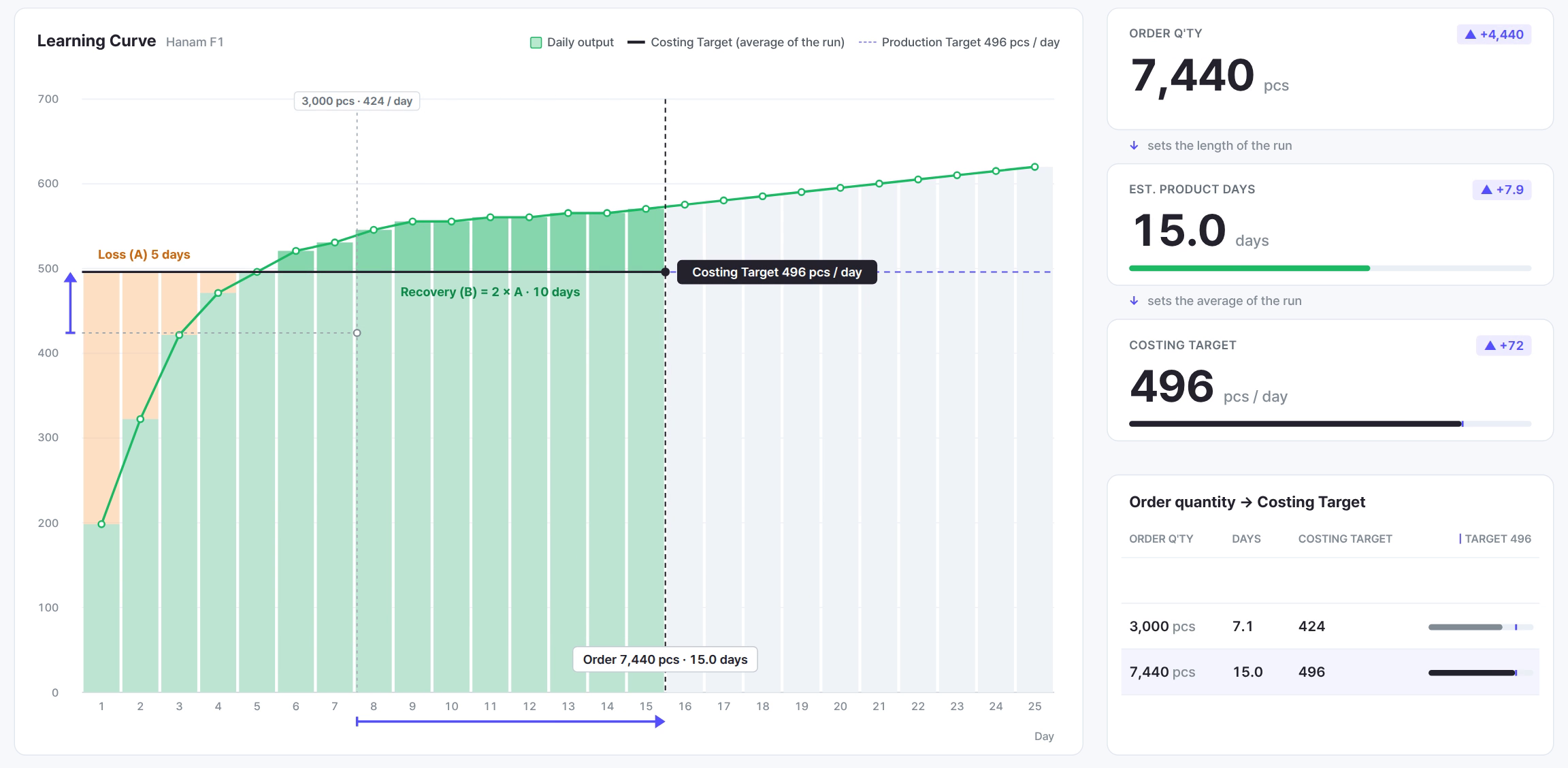
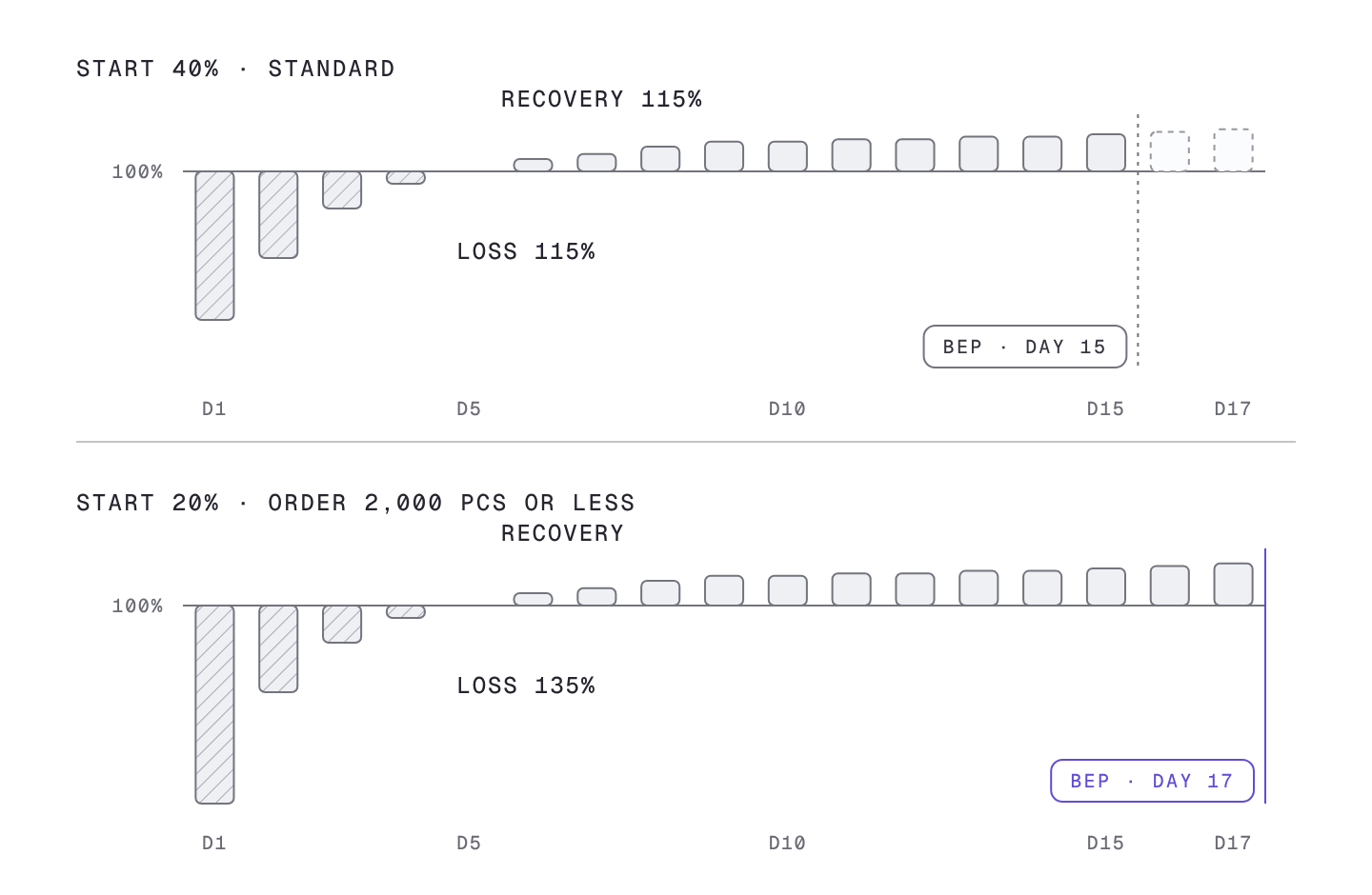
Now change only the start. Set day one at 20% instead of 40% and the day 1 shortfall grows from 60% to 80%, so the loss area becomes 80 + 35 + 15 + 5 = 135%. With 20% more to pay back, recovery takes longer and break-even moves from day 15 to day 17. A difference on a single first day pushes break-even back by two days.
The same principle applies to the figure used in quotes. Quotes use the Costing Target rather than the daily target. The Costing Target is the average daily output over the whole order, slow days included. If an order ends inside the loss zone, or the loss zone takes up a large part of the order, the average is pulled down by the loss area.
The calculation in Supplement 1 shows this. At the same daily target of 496 pcs, the Costing Target was 297 pcs for a 1,000 pcs order, 424 pcs for 3,000 pcs and 516 pcs for 10,000 pcs. A 1,000 pcs order spends most of its run in the loss zone, so the average drops a lot, while a 10,000 pcs order has a long recovery zone and more after it, so the average rises above the daily target. The CM is calculated by dividing by this Costing Target, so the larger the share of the run taken by the loss area, the higher the CM. The loss area reaches all the way to the unit price on the quote.
Inputs that change the three numbers
At this point the next question follows naturally: if the start and the reach day matter this much, what changes them? The standard curve is not a fixed table. The in-house process analysis workbook contains inputs that change the three numbers, and two of them apply automatically once the order details are entered.
Order quantity changes the start
The first input is order quantity. For orders of 2,000 pcs or less, day 1 starts at 20% instead of 40%. The workbook holds this as a condition that switches the day 1 rate the moment the order quantity is entered.
Connect this to the earlier result and the weight of the rule shows. With a 20% start the loss area grows to 135%, and because a small order spends most of its run in the loss zone, that effect passes almost straight into the Costing Target. This rule is also why Supplement 1 found that the same 1,000 pcs takes 3.1 days with a 40% day 1 and 3.4 days with 20%.
A repeat order lifts the whole curve
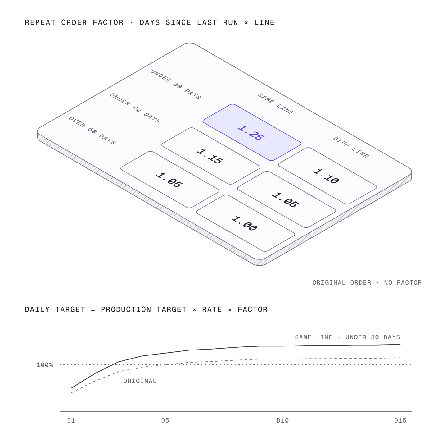
The second input is the repeat order. When the same style is produced again, the order type is chosen from three options: a style made for the first time (ORIGINAL), a rerun on the same line (REPEAT SAME LINE), and a rerun on a different line (REPEAT DIFF LINE). For a repeat order, the number of days since the last run is entered as well, and the workbook looks up the factor in the table below.
| Days since last run | Rerun on same line | Rerun on different line |
|---|---|---|
| Within 30 days | 1.25 | 1.10 |
| Within 60 days | 1.15 | 1.05 |
| Over 60 days | 1.05 | 1.00 |
The factor multiplies the daily targets directly.
Daily target = Production Target × that day’s rate × repeat factor
For a style made for the first time, no factor is applied. For a repeat order the same factor is applied from day 1 to the last day, so the whole curve moves up while keeping its shape. With higher daily targets, the Costing Target rises too.
Read the table in two directions. Across, the same line has a larger factor than a different line, because the operators who made the style are still there, and so are the attachments and the process layout set up for it. Down, the closer the rerun is to the last run, the larger the factor, because over time hands forget the motions and the chance that the line’s people have changed goes up.
For example, if the same style comes back to the same line within a month, the factor is 1.25. It is the largest value in the table, the case where the line remembers the style best. If it is made again on a different line more than two months later, the factor is 1.00, the same as a style made for the first time.
Style difficulty and factory capacity
The third group is harder to fit into a single workbook table: production difficulty driven by fabric type and design complexity, and the factory’s processing capacity driven by headcount and operating hours. SIJE patent note 2 introduced these two factors, together with order quantity, as inputs for predicting output.
The first two inputs follow clear rules and fit in a table, but difficulty and capacity combine differently for every style and factory, so a table cannot hold them all. SIJE therefore uses these two factors as inputs that redraw the standard curve, starting from the same base and setting the start and the reach day differently depending on the style and the factory.
A real factory’s curve was slower than the standard
So far we have covered the standard curve and the rules that adjust it. Next is how closely a real factory’s curve follows the standard. Answering that takes measured data.
Using more than two years of daily line output from one sewing factory in Indonesia, we calculated target attainment by working day after a new style goes in. The working day is the count of days from the day the style went on the line, and target attainment is that day’s output divided by that day’s target. The values are medians across line records. The median is the middle value when the records are sorted by size, and it keeps unusually bad days, such as a power cut or a wait for materials, from dragging the figure down the way an average would.
| Working day | Day 2 | Day 3 | Day 4 | Day 5 | Day 7 | Day 10 | Day 12 |
|---|---|---|---|---|---|---|---|
| Standard curve | 65% | 85% | 95% | 100% | 107% | 112% | 113% |
| This factory, measured | 37% | 62% | 75% | 84% | 93% | 97% | 100% |
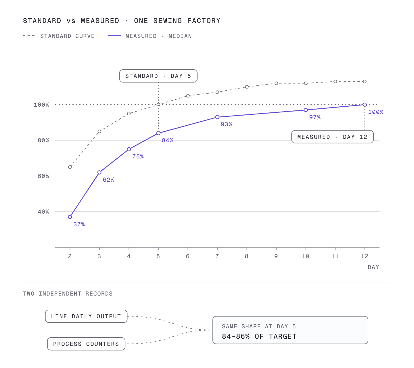
Read the table by comparing the two rows day by day. On day 2 the standard is 65% and the measured value is 37%. On day 5 the standard has already reached 100% while this factory stays at 84%. This factory reaches 100% on day 12.
Translate this into the three indicators and the difference becomes clear. The reach day moved from day 5 to day 12. The puddle is more than twice as wide, and the daily shortfall is also larger than the standard, so the loss area becomes much larger than the standard 115%. Use the standard curve as is for this factory and the Costing Target is set higher than reality, so the CM comes out lower and production days shorter. This is how a quote that looks right ends up losing money in production and slipping on schedule.
One more thing has to be checked: whether this curve is an accident of one kind of record. The factory had two kinds of records. One is the daily output written for each line, and the other is the piece count from counters on each process. The two are collected in different ways. Calculating the curve from each of them gave the same shape, at 84~86% on day 5. Just as two thermometers showing the same temperature let you trust the reading, the fact that two independent records drew the same curve is what this result rests on.
Calibrating the standard curve into a factory curve
Now we can go back to the opening question. How far can 40% on day one be trusted? Trust it and use it at the first stage of a quote, and correct it once the factory’s own records build up.
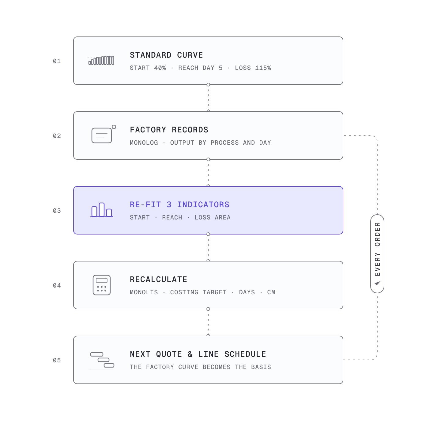
Calibration works through the three indicators. From the factory’s records, find the start, the reach day and the loss area again, and redraw the curve with those values. When the curve changes, the Costing Target changes, and when the Costing Target changes, the CM and production days follow. It is the move from the standard curve to the factory’s own curve.
The problem is that this calibration is hard to do by hand. Getting a single curve means collecting daily output by style and line, finding the start date and recounting working days, filtering out unusually bad days, and then sorting by day. Splitting it by order quantity, repeat status and style difficulty means repeating the whole job for each condition. With that much work, it is easy to fall back on the standard curve as it is.
On lines with Monolog installed, output by process builds up automatically, so this calibration can keep running without separate work. Monolis recalculates the Costing Target and production days with the calibrated curve and feeds them into the quote and the line schedule. Factory records become a curve, and that curve becomes the basis for the next order’s quote. This process is part of what SIJE calls turning manufacturing knowledge into an asset.
Summary
| Indicator | Meaning | Standard curve | Inputs that change it |
|---|---|---|---|
| Start | Share of the daily target made on day 1 | 40% | Order quantity (20% for 2,000 pcs or less) |
| Reach day | First day at 100% | Day 5 | Style difficulty, factory capacity, measured calibration |
| Loss area | Total shortfall against target | 115% (135% with a 20% start) | Start and reach day, repeat order factor |
40% on day one is a starting value set so that quotes can begin from the same numbers. Read the loss zone as start, reach day and loss area, and you can see where that starting value needs correcting, and the curve corrected with each factory’s measured data becomes the basis for quotes and schedules.
Related: Why the First Week Loses Money: Putting the Learning Curve into the Quote
Related: SIJE Patent Note (2): Small-Batch Production and AI Prediction
